Exploring VJEPA’s latent space

Since their release a couple of weeks ago, I’ve been curious about the new V-JEPA 2.1 models and their capabilities. Because of how they are trained, they build rich semantic and temporal representations of video in a latent embedding space.

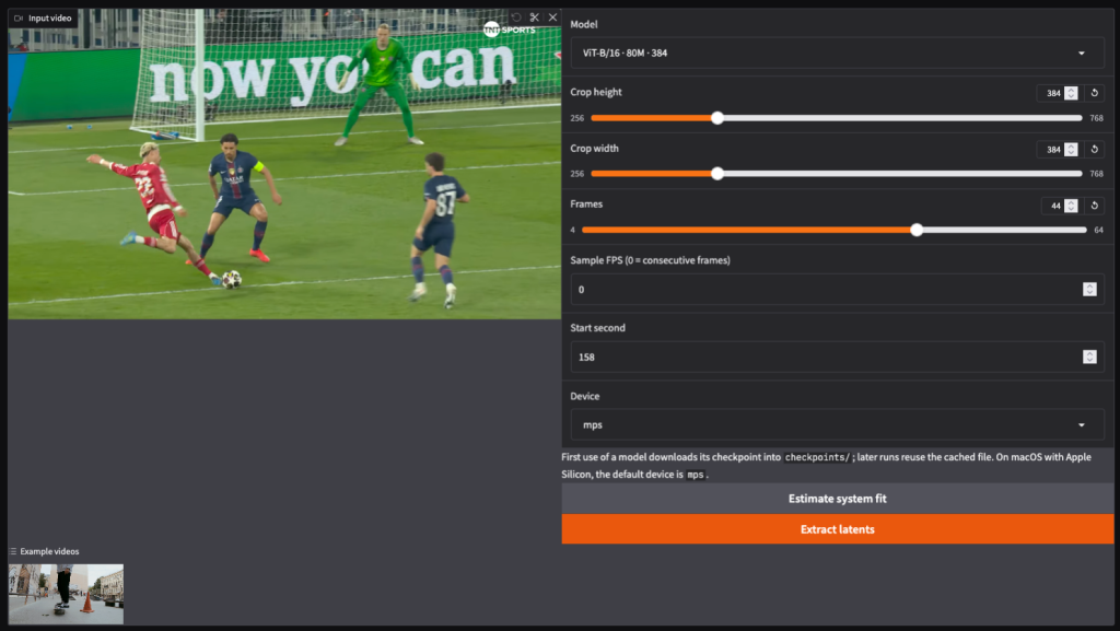
To briefly break down how the model works: if we feed the model 44 frames of a 384×384 video, it outputs 12,672 tokens of 786 dimensions each, the 44 frames collapse into 22 time slices (2 consecutive frames per slice), and the 384×384 resolution is split into a 24×24 grid of 16×16 pixel patches (22×24×24=12,672).

If we’re using the 80M parameter model, each token is a 768-dimensional vector (larger models output larger dimensions). Essentially, every single token is a compressed representation of a specific 16×16 patch spanning two consecutive frames. In addition each output token for a patch has attended to other patches in the same time slice and other time slices forward and backward in time in the video sequence.

I wanted to create a playground to intuitively probe this latent space. What I have so far is a Gradio app that takes in a video, lets the user tweak the frame count and crop size, and feeds it directly into the model.

Dimensionality Reduction: Visualizing the Latent Space

To better understand the shape of the V-JEPA latent space, the first statistical tools I reached for were dimensionality reduction techniques like PCA and UMAP.

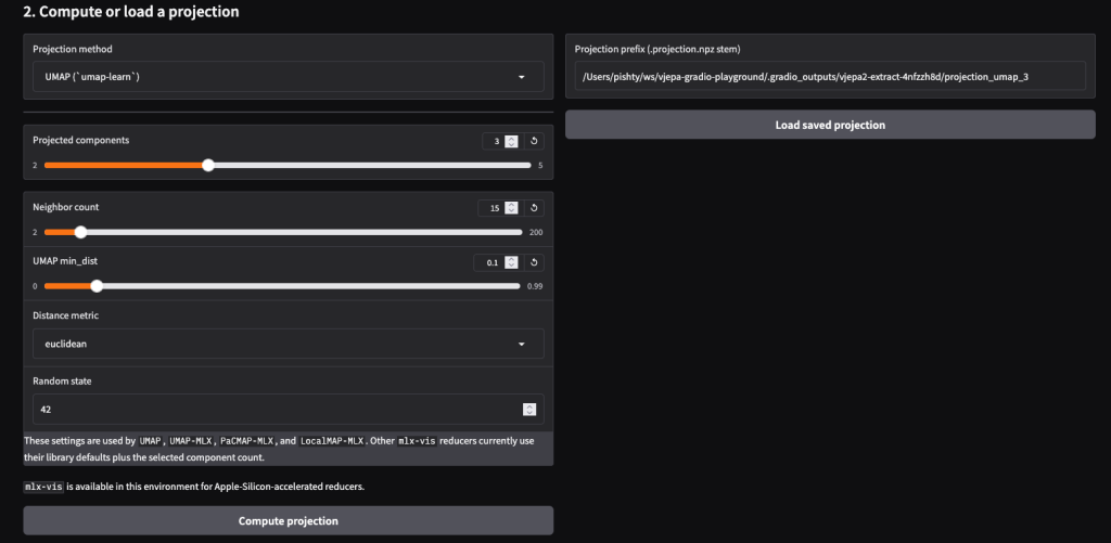
By reducing the high-dimensional feature vectors (768 dimensions) down to just 3, we can plot each video token in a 3D scatter plot and track how those points behave across the sequence of frames. Doing this revealed a few interesting observations and raised some new questions:

• Observation 1: UMAP > PCA. UMAP produces much more visually distinct and interesting structures than PCA. This makes sense, as UMAP is better at capturing complex, non-linear relationships in high-dimensional data, whereas PCA is strictly linear.
• Observation 2: Semantics over Position. When looking at the UMAP plot across 22 time slices, the prominent clusters remain surprisingly stable. Even when objects are actively moving across the screen, the groupings hold their shape. This leads me to conclude that these clusters represent the semantic meaning of the objects (e.g., “this is a car”, “this is the road”) rather than their exact spatial positions.
• Observation 3: Pushing the limits of visualization. Currently, we are reducing each token to 3 dimensions to plot them in 3D space (X, Y, Z). However, we could theoretically reduce the data to 7 dimensions and still visualize it in a single plot: 3 dimensions for the spatial coordinates, 3 dimensions mapped to RGB colors, and 1 dimension for opacity. It would make for a wildly colorful—if potentially chaotic—visualization!

Visualizing the data like this builds our intuition. Once we know that the model naturally clusters semantic meaning together regardless of movement, it opens the door to powerful downstream applications—like zero-shot dense object tracking and video segmentation.

Painting with Data: Mapping the Latent Space to RGB

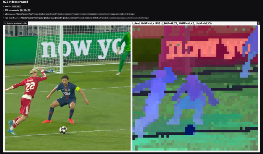
The second major advantage of reducing our tokens to three dimensions is that it perfectly aligns with the three color channels of standard displays: Red, Green, and Blue (RGB).

By mapping our X, Y, and Z coordinates directly to R, G, and B values, we can assign a specific color to every single token. Since each token represents a 16×16 spatial patch from the original video, we can stitch these colored patches back together to construct an entirely new video.

This technique is incredibly powerful because it gives us a literal, color-coded map of how the model semantically understands the scene. Patches that share similar semantic meaning cluster together in the 3D latent space, which means they end up being painted with very similar RGB colors.

As we can see from the side-by-side comparison below, the results are striking. Without being explicitly trained to track or segment anything in this football clip, the model’s internal representation naturally distinguishes between the distinct elements of the scene. It flawlessly separates the ball (dark blue), the lines on the pitch (dark horizontal bands), the lettering on the background advertising board (pinkish-red), and of course, the players themselves (light blue and purple).

Zero-Shot Object Tracking via Patch Similarity

Since our UMAP visualizations proved that the model assigns a consistent mathematical signature to objects across different frames, we can actually leverage this to track objects over time.

Instead of relying on the reduced 3D visualizations, we can go back to the raw, high-dimensional latent tokens (all 768 dimensions) and compare them mathematically using Cosine Similarity. The logic is simple: if we select a specific patch in the first frame—for instance, the football—we can measure its cosine similarity against every single token in the subsequent frames. The token with the highest similarity score is our target.

To test this, I built a dense tracking interface. As shown in the screenshot below, you simply click on an object in the original video (the red square on the left). The tool then computes the similarities and generates a heatmap overlay on the video (on the right). Without any fine-tuning or traditional object-detection algorithms, the model successfully tracks the ball as it moves across the pitch.

The Tumbling Window Experiment

While building out this UI and poking around the V-JEPA 2.1 latent space, I confirmed something expected: the model is perfectly deterministic. If you feed the exact same video clip into the encoder multiple times, you get the exact same matrix of numbers out.

But this led me to a much more interesting question: What happens if we feed the model two clips that are almost identical, but shifted slightly in time?

To test this, I built a Tumbling Window comparison tool.

Before looking at the results, there is one crucial detail to understand about V-JEPA: it processes video in 2-frame chunks called tubelets. This means the model takes frames in, but spits latent time slices out.

Let’s look at a simple sliding window experiment starting at Frame 1, using 20-frame clips:

• Run A (First Window): Inputs Frames 1 to 20 (Outputs 10 time slices)
• Run B (Second Window): Inputs Frames 3 to 22 (Outputs 10 time slices)

The Overlap: Frames 3 through 20 are visually identical in both runs. Because they span 18 frames, this gives us exactly 9 overlapping time slices.

While the pixels in this overlap are exactly the same, their temporal context has changed. For example, Frames 3 & 4 make up the second time slice in Run A, but they make up the very first time slice in Run B.

Does the model assign the exact same internal representation to these shared time slices? Or does the surrounding context alter how they are encoded?

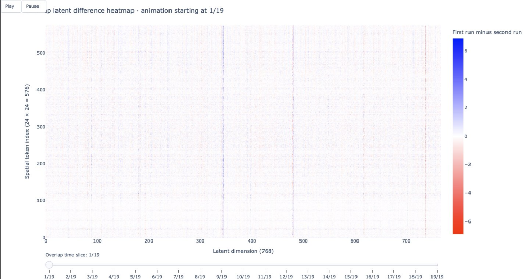
To find out, I subtracted the latent matrix of Run B from Run A for each shared time slice, and mapped the differences onto an animated heatmap.

• The X-axis represents the 768 dimensions of the latent feature vector.
• The Y-axis represents the 576 spatial patches (a 24×24 grid representing the image for that specific time slice).
• White pixels mean the vectors are mathematically identical (a difference of zero).
• Red and Blue pixels indicate a mathematical difference between the two runs.

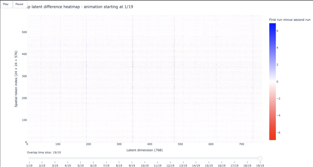
Here is what the overlap looks like at the beginning, middle, and end of the shared time steps (40 frames windows i.e. 20 time slices with 19 shared time slices:

1. The First Shared Time Slice (Slice 1 of 19):At the start of the overlap, we see a noticeable amount of red and blue noise. Even though the input pixels are identical, the model encodes them differently.

2. The Middle Shared Time Slice (Slice 10 of 19): As we move to the middle of the shared sequence, the heatmap goes almost completely white. The differences vanish. The model is encoding these frames virtually identically across both runs.

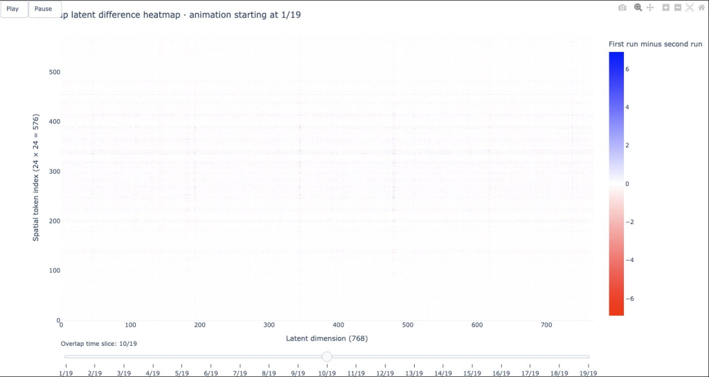
3. The Last Shared Time Slice (Slice 19 of 19): At the very end of the overlap, the red and blue differences emerge once again.

Bidirectional Context

The heat maps illustrate how V-JEPA thinks about time. Unlike a language model (like ChatGPT) which only looks backward at the words you’ve already typed, the V-JEPA encoder uses Global Bidirectional Self-Attention. Every single patch in the video sequence looks at every other patch—both backward into the past, and forward into the future—to build its final representation.

This explains the heatmaps perfectly:

• The Edges (Slices 1 and 19): Let’s look at Slice 1 (Frames 3 & 4). In Run A, this slice can look backward at Frames 1 & 2 for context. In Run B, it is the very first slice, so it is blind to the past. Because their available contexts are asymmetrical, the Transformer calculates slightly different mathematical features.
• The Middle (Slice 10): By the time we reach the middle slices, the patches have plenty of context looking backward AND forward in both runs. Because the surrounding context is functionally identical in both directions, the math converges, and the output is exactly the same (almost pure white).

The Temporal Fingerprint: High-Sensitivity Dimensions

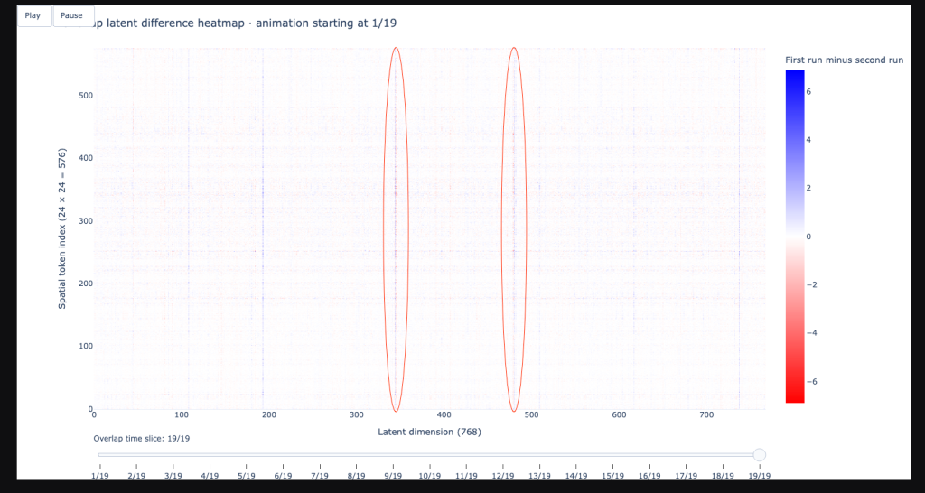
Beyond the overall shift in context, I noticed a very peculiar pattern that appeared regardless of which video I used. In the Tumbling Window heatmaps, certain vertical columns almost always light up with intense red or blue values at the edges of the overlap (the first and last shared time slices).

Because the X-axis represents the 768 individual dimensions of the latent space, these vertical streaks tell us that specific feature channels are hyper-sensitive to temporal positioning.

Even when the visual content changes entirely—from a football match to a nature documentary—these specific dimensions (highlighted in the red circles above) consistently show a large mathematical delta when their position in the window shifts.

This is a fascinating peek into the brain of the model. It suggests that V-JEPA 2.1 has specialized dimensions essentially temporal specialists whose primary job is to track the relative position of a frame within a clip. When we shift the window, these specific channels are the first to notice that their context has changed, even if the semantic meaning of the objects in the frame stays exactly the same.

Wrap-up

All the visualizations, heatmaps, and tracking experiments shown in this post were generated using the V-JEPA 2.1 Latent Explorer.

Key features include:

• Latent Extraction: Reusable artifacts (.npy and metadata) for deep analysis.
• Memory Management: Automatic pressure estimation for local GPUs.
• Dimensionality Reduction: Built-in PCA and UMAP pipelines.
• Interactive Visuals: 3D Plotly views and RGB-mapped latent videos.
• Downstream Tasks: Ready-to-use workflows for object tracking and tumbling window experiments.

The latent space of V-JEPA 2.1 is incredibly rich, and we are only just beginning to scratch the surface of what these world model representations can do.

Source code vjepa-latent-explorer on GitHub